PHOENIX

Introduction[]

Modern science uses computers in many different ways - to control experiments, to acquire and analyse data and to perform mathematical modeling and simulations. Using a PC to interact with the real-world (say take temperature measurements, read fast changing voltages) is not a difficult job for a person well versed in electronics and computer programming - but it can be daunting for a school/college student who is just beginning her journey into the wonderful world of science and technology. The objective of the Phoenix project is to reduce this barrier to entry significantly by developing a low-cost, microcontroller based interfacing device and associated software. Using Phoenix and a PC loaded with GNU/Linux and other free software, students can interact with real world phenomenon by writing short programs (often just two or three lines of code) in a simple, easy to learn language called Python. Because it is based on a Microcontroller (the Atmel ATMega16), the Phoenix box can also be used for studying embedded systems development.

Phoenix is being actively developed by the Inter-University Accelerator Centre, New Delhi. IUAC is an autonomous research institute of University Grants Commission, India, providing particle accelerator based research facilities to the Universities. For more information regarding Phoenix, visit the official home page at http://nsc.res.in/~elab/phoenix/.

The developers of Phoenix believe in the power of free knowledge - the whole of Phoenix, including the circuit schematics and the software is available for study, modification and sharing by the community. The software (both the firmware running on the microcontroller which forms the `brain' of Phoenix and the interface code written in Python and running on the PC under GNU/Linux) is licensed under the GNU GPL. Electronics hobbyists, free software and science enthusiasts are encouraged to play with Phoenix, design new experiments and extend its hardware and software. This wiki is intended to become a repository of all contributions to the project by the community

Experiments Developed by the Community[]

This section is devoted to experiments developed by the community.

Developing a Phoenix-M plugin - DTMF encoder UM91214[]

The Phoenix box comes with a 16 pin LCD connector through which we can access the following pins of the ATMega16 microcontroller - PD4, PD3, PD2 (of PORTD) and PA4, PA5, PA6, PA7 (of PORTA).

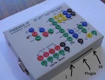
Here is how the LCD connector pins are mapped to the port pins: pins 4,5,6,11,12,13,14 of the LCD connector are mapped to PD4, PD3, PD2, PA4, PA5, PA6, PA7 respectively. Pins 2 and 1 of the LCD connector slot are respectively +5V and GND.

These pins can be used for developing `plug-ins' which enhance the functionality of the base unit. Already developed plug-ins include a high-resolution AD/DA card and a serial EEPROM interface (more info at http://nsc.res.in/%7Eelab/phoenix/plugins/index.html). In this experiment, we will see how easy it is to develop a plug-in for Phoenix-M!

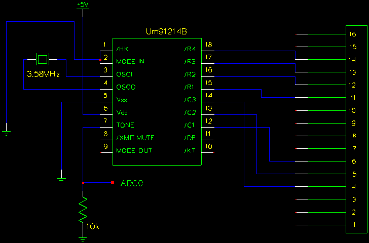
Here is a schematic of the UM91214B (a DTMF encoder chip) interfaced to the LCD connector pins:Media:Dtmf-plugin.png. You can read more about DTMF here. The UM91214 helps you to combine two sine-waves of different frequencies (a low and a high - both less than 2KHz) - the resulting waveform can be digitized using the Phoenix-M ADC - it can also be subjected to further mathematical processing (say taking the Fast Fourier Transform) on the PC. It is possible to determine the two component frequencies using Digital Signal Processing techniques - in this case, I have written a small program which uses the Python FFT library to look at the frequency spectrum of the waveform produced by the UM91214. The FFT is useful for examining a range of frequencies - detecting one particular frequency is better done using the Goertzel Algorithm.

The LCD connector pins (to which the UM91214 is interfaced) are used to control the lines R1, R2, R3, R4 and C1, C2, C3. If say R1 is low and C1 is low, the tone output (from pin 7) is 697 + 1209 Hz. Other combinations produce different tones. An FFT will show peaks in those frequency bands containing these tones.

Developing a plug-in requires modifying two files: avrk.c and phm.py. The first file is compiled to get the firmware which is loaded into the ATMega16 microcontroller and the second file is the Python library using which we interact with the code running on the controller.

The way the Python library interacts with the code running on the microcontroller is as follows: say we wish to read the logic levels on the 4 digital input pins. What we do is simply type:

p.read_inputs()

The read_inputs function sends out a command DIGIN (which is mapped to a number, in the current version of the Phoenix code, it is 2) through the serial port. The code running on the ATMega16 reads this number, stores it into a buffer (called par.buf) and increments an index (called par.buf_index, it's initial value is zero). Now, a command (from the PC to the controller) can be followed by one or more arguments. Say we wish to write a value to the digital output pins - in that case, the command to write a value should be followed by the value to be written. There are different types of commands depending on the number of arguments each one takes - the first set is the set of all commands which take no arguments (like DIGIN) - there can be a maximum of 40 such commands, numbered 1 to 40. The second is the set of all commands with one argument (like DIGOUT) numbered 41 to 80 and so on ... After determining that the command and all its arguments have been received properly, the main routine in avrk.c calls the function processCommandwhich looks at the command number and executes a BIG switch statement (which is the core of the code in avrk.c). Here is the fragment of code corresponding to a DIGIN:

processCommand()
{
     tmp8 = par.buf[0];
     par.buf[0] = DONE;
     par.buf_index = 1;
     switch(tmp8) {
          ........
          ........
           case DIGIN:
              par.buf[par.buf_index++] = PINC & 15;
              break;
           /* Other cases .... */
     }
}

The function replaces par.buf[0] with a return code DONE (indicating success) and then DIGIN stores the value read from the port in the next slot of the array. Once control breaks out of the switch, a simple for loop writes all items from par.buf[0] to par.buf[par.buf_index-1] to the serial port which will then be received by the Python code running on the PC.

Here are the modifications we make to avrk.c for our DTMF plugin. We first define a new command DTMFOUT (command number 62, belongs to set of all commands taking one argument).

#define DTMFOUT 62

Then we add the following fragment of code to avrk.c:

 case DTMFOUT:
    
    // LSB 4 bits of data contains row number and MSB 4 bits column
    // number,
      
       tmp8 = par.buf[1];
      
    // R1, R2, R3, R4 on PA4, PA5, PA6, PA7 and
    // C1, C2, C3 on PD2, PD3, PD4.
      
       DDRA = DDRA | 0xf0;
       DDRD = DDRD | 0x1c;
       PORTA = PORTA | 0xf0;
       PORTD = PORTD | 0x1c;
       delay_us(10000);
       PORTA = PORTA & ~(1 << (3 + (tmp8 & 15)));
       PORTD = PORTD & ~(1 << (1 + ((tmp8 >> 4)&15)));
       delay_us(10000);
       
       break;

The command accepts a one byte argument - the LSB 4 bits is a row number (ie, whether we want to activate R1, R2, R3 or R4) and the MSB 4 bits is a column number (ie, whether we want to activate C1, C2 or C3). The code simply configures the corresponding port pins as outputs, writes a 1 to all the pins, waits for some time and then writes zero's to ONLY the row and column to be activated. This results in the DTMF chip generating a tone with two frequencies combined (read either the chip manual or wikipedia entry on DTMF to know more about the frequency combinations).

Here is the code added to phm.py (the Python interface library):

	def dtmf_out(self, row, col):
		""" Generates DTMF pulse corresponding to
                a key press in row/col.
		"""

		dat = (col << 4) + row
		self.fd.write(chr(DTMFOUT))
		self.fd.write(chr(dat))
		self.fd.read()
		return

The code simply combines the row/column numbers into a one byte argument and sends it after the command DTMFOUT. The self.fd.read before the return statement simply reads and ignores the DONE output transmitted by the microcontroller. We need to add more error checking to both avrk.c and phm.py!

You can download a .tgz file containing avrk.c, phm.py and spectrum.py (a simple program which reads in the tone output and performs an FFT and displays the output) from here

Observing TV refresh using a Phototransistor[]

Look at the following circuit:

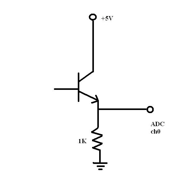
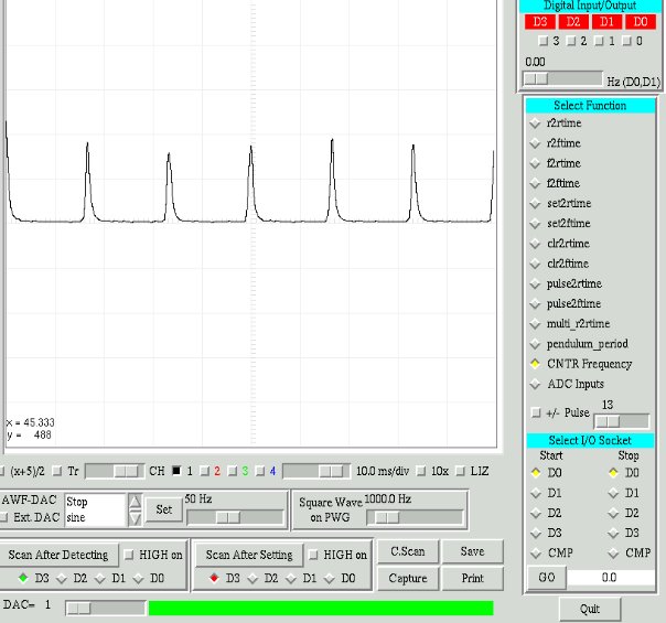
I observed the voltage across the resistor using the CROPlus utility. Here is what I got:Media:Crt2.jpg.

Images are generated on the TV screen by an electron beam which lights up pixels one after the other. Once all the pixels are illuminated, the process repeats; as many as about 60 times per second. A phototransistor placed very close to the monitor picks up these periods of brightness easily.

When the voltage across the resistor was given to the CNTR input and the CROPlus utility was used to measure frequency, I consistently got a reading of 60Hz.

If we keep one phototransistor at the top left corner of the screen and another one at some other place, will it be possible to infer the position of the second one by the difference in time it takes for the electron beam to illuminate the area under both? A good exercise to try out!

Transistor Characteristics[]

This experiment is to study the different characteristics of a transistor such as transfer characterisitics (output voltage vs input voltage), input characteristics (input current vs input voltage) and output characteristics (output current vs output vltage). The standard results are given in all electronics text books. The circuit used here has a fixed bias on the collector side and only the base voltage is varied. So, our output characteristic curve is actually the load line. Besides, the input characteristic is not measured keeping the collector voltage constant. So it doesn't make much sense to study the input and output curves at this point. To obtain the whole set of curves, the collector bias needs to be varied as well, and requires two DAC's. I'll try to get a plug-in DAC and update as soon as possible.

Now, the transfer characteristics can be studied quite accurately. We should expect a straight line, obviously, for the transistor to act as an amplifier. If the curve is not linear, the amplified signal would be distorted.

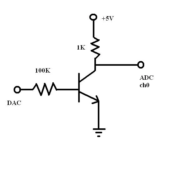
The circuit is set up as shown above. Now, the input voltage (DAC) can be programmed to vary from 0-5000 mV in steps of 20 mV. For each value of input the output is measured using the ADC channel 0.

                #transistor.py

import phm
p = phm.phm()
p.select_adc(0)
m = 0
while(m<5000):
	p.set_voltage(m)
	n = p.zero_to_5000()
	print m,n[1]
	m = m+20

The data can be redirected to a file and plotted using gnuplot.

HAVE FUN WITH ELECTROMAGNETICS!!![]

Here is a simple example of how you can play with electromagnetic waves. Hook up a 10 cm long piece of ordinary wire to the Programmable Waveform Generator (PWG) socket of your Phoenix-M. Tune your radio set to 1 MHz(any other frequency in the Medium Wave band, for easy reception with an ordinary radio set, if there is a radio station nearby at 1 MHz), and keep it nearby. You would hear a lot of noise. Now, run the following code fragment, which sets the PWG to a 0-5V 1 MHz square wave.

import phm
p=phm.phm()
p.set_frequency(1000000)

You would observe that the noise has disappeared! When I did this experiment, I got a constant high-pitched hum, probably due to some constant audio-frequency noise being produced during the waveform generation. Anyway, you would be able to observe the absence of the random noise, quite clearly, which means the signal is being received by the radio. Now change the frequency at the PWG to, say 100 Hz.

p.set_frequency(100)

You would hear the noise again, instantaneously. Next, run the following loop, to switch the signal frequency between 100 Hz and 1 MHz every second.

import time
while(1):
     p.set_frequency(1000000)
     time.sleep(1)
     p.set_frequency(100)
     time.sleep(1)

The noise would go on and off every second, according to the frequency of the signal. You have built your own crude radio-frequency digital data transmitter!!! You can develop a protocol to interpret and send data, just using the on/off signal!

The electromagnetic waves produced by the voltage oscillations (0-5V) in the wire, can be detected across a distance of about 3 m. That's simply amazing, considering the fact that we are switching between only 0-5V, and the antenna we have used is just a small piece of ordinary wire!

Documentation[]

How to add custom files to your live CD[]

SLAX CD contains a directory /rootcopy/. The content of this directory is copied to root filesystem each time you boot SLAX, preserving all directories.So, for example, if you want to add a file book.pdf to the /home/guest/ directory,

1.Copy the contents of the live CD into a directory.

2.cd to that directory, and then to rootcopy/

3.rootcopy/ would be empty by default, so create a directory rootcopy/home/ and then rootcopy/home/guest/. Now copy book.pdf to rootcopy/home/guest/.

4. Make the iso image of the modified CD- cd to the directory where the contents of the CD are copied, and-

./make_iso.sh /tmp/phm_new.iso

5. Burn the image on a blank CD, and your files will be present in the new CD, at the desired location.

How to add a new tool to your LIVE CD[]

1. Get the .tgz package of the tool you want to add, for the appropriate version of slackware, from http://linuxpackages.net and save it on your hard disk.

2. Boot from your live CD and mount the hard disk. cd to the location where you saved the package, and convert the .tgz package to a slax module using the command-

tgz2mo [.tgz (source) filename] [.mo (target) filename]

3. Now copy the contents of the live CD into a directory and add the .mo file you created in the previous step, to the /modules/ directory of the CD.

4. Make the iso image of the modified CD as directed above.

5. Burn image.

Note:- You should know the libraries which the software depends on. And when copying libraries (you can use rootcopy), you should take care to copy both the symbolic link, and the actual library.

Courtesy:http://slax.org

Project Ideas[]

Share your thoughts about what you can do with Phoenix.

Projects for School students[]

Projects which school students would be able to understand and appreciate.

Human response time - program lights an LED and we close a switch when we see the LED lighting up - program measures time.
How fast can we move our hand? Two light sensors should do the job.
Human response time. Time you take to close a switch after seeing an LED turning ON. very simple, set2ftime() call
Timing a race
How do computer input/output devices work?
1. Reading a simple switch
2. A potentiometer based joystick
3. A matrix keyboard
4. Generate signals to drive a TV
5. Light sensor (phototransistor) demonstrates TV refresh
6. Can we use two phototransistors to build some kind of a light pen?

New Experiment

Advocacy[]

How can we involve more people in the development of Phoenix? How can we use Phoenix as an aid for teaching science, programming, computer interfacing .... Share your thoughts.

Summer workshop for school students[]

Students will be in holiday mood ... how to catch hold of them and make them do something creative with Phoenix?

Tentative Syllabus for Basic Electronics Session[]

BASIC COMPONENTS
- BATTERY-source of power

Let's start off by showing students how to use a multimeter to measure voltage. Let's not go into abstract discussions of what exactly voltage is - we will just say that its something similar to `force' - a kind of force which results in work being done in an electronic circuit.

- LED-light emitting device

Let's show students perhaps the cutest of all electronic components - the LED! We will just demonstrate an LED lighting up when connected to a battery - we will not at this point introduce the idea that we have to limit the current through the circuit.

- Controlling current through the circuit-RESISTOR

Use a 2.2K resistor in series with the LED. Use a 470 Ohm in series. Ask the students to note the difference in brightness. Provide a very rough idea as to what `current' really means.

- - colour coding

Teach students how to read color codes - ask them to verify using multimeter.

- variable resistor-
  - POTENTIOMETER
  - LDR

This will be an interesting demo - ask students to measure resistance of an LDR under different conditions of illumination.

- - PHOTOTRANSISTOR -
- CAPACITOR-store charge. Should we have a demo here? Let's look at how the students are responding and then decide.

- SPEAKER/MIKE-convert voltage to sound and vice versa - there is no way we can have a demo here - will do the demo after Phoenix is introduced.
- need for constant voltage supply-VOLTAGE REGULATOR
  - 7805 demo - introduce circuit contruction on breadboards.

- DIODE-conducts only in one direction. Shall we do a demo?
- TRANSISTOR-as a switch.
- IC-familiarization.

RESISTOR NETWORKS
- Series/Parallel
- Hands on- Measure resistance of series/parallel combinations of resistors and frame an inference. Before doing measurement with a multimeter, let the students see the effect of adding resistors in series and parallel on an LED - that will be interesting.
  - Series-equivalent resistance is greater than each individual resistance
  - Parallel-equivalent resistance is less than each individual resistance

OHM'S LAW
- Current-Voltage relation, V/R = I
- voltage dividers. Again, rather than explaining a formula, let students do measurements and form their own inference. Let the formula reinforce ideas which have been gained intuitively and experimentally.

Demo of an interesting circuit (a)- the highly sensitive charge detector!
Demo of an interesting circuit (b)- Measure room temperature with LM35 sensor!

- - Hands on-
    1. 555 timer circuit- blinking LED. Don't explain theory. Just let the students gain some experience constructing a circuit on a breadboard.
- PCB - Some idea about how PCB's are manufactured.
- Common PCB

PROJECT-to be updated later

Events[]

Please add events at which the Phoenix project will be represented here.

1. A 2 day workshop on using PHOENIX for physics experiments was held at the Midnapore College, Midnapore, West Bengal on the 17th and 18th of March, 2007.

2. A 3 day workshop for school students at Tharakan high school, Angadipuram from 29 April to 1 May.

3.Demo and talk on the PHOENIX and its development ideas by Ajith Kumar and Pramode C E at Vidya Academy of Science and Technology, Thrissur on June 11 2007.

How to make a Phoenix Live CD from a Debian Installation[]

See this page for instructions.